Classical vs. Learned Image Segmentation

This project, developed with Marcos Levi Pinto Sousa at ITA, compares two very different approaches to binary semantic segmentation: the classical, energy-based GrabCut algorithm and a lightweight U-Net implemented from scratch in PyTorch.

Both methods were evaluated on the same validation subset of the Oxford-IIIT Pet Dataset. The objective was not only to measure which method produced better masks, but to understand what that improvement costs in training time, model state, and computational resources.

Formally, both methods estimate a binary labelling function

$$f : \mathbb{R}^{3 \times H \times W} \longrightarrow \{0,1\}^{H \times W}, \qquad \hat{Y}=f(X) \tag{1}$$

but they arrive there through different assumptions. GrabCut infers the mask for each image by fitting a probabilistic color model and optimizing an energy. The U-Net learns the parameters of a nonlinear function from many labelled examples, then applies that function directly at inference time.

Results at a glance

Pixel accuracy

GrabCut0.76 ± 0.17

U-Net0.87 ± 0.08

Intersection over Union

GrabCut0.58 ± 0.23

U-Net0.74 ± 0.14

+11 ppaccuracy

+16 ppIoU

−0.09IoU spread

The learned model improved pixel accuracy by 11 percentage points and IoU by 16 points. Its lower standard deviation also indicates more consistent performance across the validation images. GrabCut, however, required neither a training phase nor a saved model, which remains a meaningful advantage on constrained systems.

Relative to GrabCut, this corresponds to approximately $14.5\%$ higher pixel accuracy and $27.6\%$ higher IoU. The larger relative gain in IoU matters: the network did not merely classify more background pixels correctly; it recovered the foreground region more faithfully.

Preparing a common task

The Oxford-IIIT Pet Dataset contains images of 37 cat and dog breeds with pixel-level trimap annotations. For this experiment, each image and mask was resized to $128 \times 128$, and the trimap was converted into a binary pet-versus-background target.

Let $X_i \in [0,1]^{3\times128\times128}$ denote an RGB image and $Y_i \in \{0,1\}^{1\times128\times128}$ its target mask. The same validation samples and target conversion were used for both methods, so the comparison changes the segmentation mechanism rather than the evaluation data.

img = self.resize(img)
img = self.to_tensor(img)

mask = cv2.resize(
    np.array(mask, dtype=np.uint8),
    (self.image_size, self.image_size),
    interpolation=cv2.INTER_NEAREST,
)
mask = (mask != 2).astype(np.float32)

Bilinear interpolation is appropriate for RGB images, but it would create invalid intermediate labels in a segmentation mask. The nearest-neighbour interpolation used for the mask preserves its discrete classes. The loader then converts every sample into an RGB tensor and a single-channel binary target.

The experiment used an 80/20 dataset split. The network was trained only on the first partition; GrabCut required no training and was run directly on the shared validation partition. This distinction is central to the comparison: the learned method pays an up-front optimization cost, whereas the classical method performs optimization independently for every image.

Classical segmentation with GrabCut

For an image with pixel colors $z=(z_1,\ldots,z_N)$, GrabCut assigns each pixel a label $\alpha_n\in\{0,1\}$ and a Gaussian-mixture component $k_n$. Foreground and background are represented by separate Gaussian mixture models with parameters $\theta=(\pi,\mu,\Sigma)$.

The segmentation is obtained by minimizing

$$\begin{aligned} E(\alpha,k,\theta,z) &= U(\alpha,k,\theta,z)+V(\alpha,z),\\[2mm] U(\alpha,k,\theta,z) &= \sum_{n=1}^{N}D(\alpha_n,k_n,\theta,z_n) \end{aligned} \tag{2}$$

The data cost is the negative log-likelihood of the pixel under its assigned Gaussian component:

$$\begin{aligned} D(\alpha_n,k_n,\theta,z_n) ={}&-\log \pi(\alpha_n,k_n) +\frac{1}{2}\log\det\Sigma_{\alpha_n,k_n}\\ &+\frac{1}{2}(z_n-\mu_{\alpha_n,k_n})^\top \Sigma_{\alpha_n,k_n}^{-1} (z_n-\mu_{\alpha_n,k_n}) \end{aligned} \tag{3}$$

Thus a pixel is inexpensive when its color is probable under the selected foreground or background component. Color likelihood alone would produce a noisy mask, so GrabCut adds a pairwise smoothness term over neighbouring pixels $\mathcal C$:

$$V(\alpha,z)= \gamma\sum_{(m,n)\in\mathcal C} [\alpha_m\neq\alpha_n] \exp\!\left(-\beta\lVert z_m-z_n\rVert^2\right) \tag{4}$$

The indicator penalizes a boundary between similar neighbours, while allowing a boundary more readily where the image itself has a strong color discontinuity. With the GMM parameters fixed, this binary energy can be minimized by an $s$-$t$ min-cut. GrabCut alternates that cut with re-estimation of the mixture assignments and parameters until the mask stabilizes.

The implementation initializes GrabCut with a bounding box derived from the ground-truth mask and expanded by ten pixels:

def get_bbox_from_mask(mask, pad=10):
    ys, xs = np.where(mask)
    height, width = mask.shape

    y0, y1 = ys.min(), ys.max()
    x0, x1 = xs.min(), xs.max()

    return (
        max(x0 - pad, 0),
        max(y0 - pad, 0),
        min(x1 + pad, width - 1) - max(x0 - pad, 0),
        min(y1 + pad, height - 1) - max(y0 - pad, 0),
    )

That initialization gives the algorithm an approximate object location without revealing the complete segmentation. OpenCV then performs five iterations and returns pixels classified as definite or probable foreground:

cv2.grabCut(
    img_bgr,
    mask,
    rect,
    bgd,
    fgd,
    iterCount=5,
    mode=cv2.GC_INIT_WITH_RECT,
)

result = (mask == cv2.GC_FGD) | (mask == cv2.GC_PR_FGD)

A $3 \times 3$ morphological opening followed by closing removes isolated noise and fills small gaps in the resulting binary mask.

An important methodological detail is that the bounding box is computed from the reference annotation. GrabCut therefore receives useful localization information that would need to come from a user or detector in a deployed system. It does not receive the final boundary, but the experiment is not evaluating fully automatic object discovery.

A compact U-Net

The learned approach uses a deliberately small encoder-decoder. Three encoder stages increase the channel count from 16 to 64 while reducing spatial resolution. Two decoder stages restore the original resolution and concatenate encoder activations through skip connections.

class UNet(nn.Module):
    def __init__(self, in_channels=3, out_channels=1):
        super().__init__()
        self.enc1 = DoubleConv(in_channels, 16)
        self.enc2 = DownSample(16, 32)
        self.enc3 = DownSample(32, 64)

        self.up3 = UpSample(64, 32, 32)
        self.up2 = UpSample(32, 16, 16)

        self.outc = nn.Conv2d(16, out_channels, kernel_size=1)
        self.activation = nn.Sigmoid()

The skip connection is the essential detail. Downsampling gives the network broader context but removes fine spatial information. Concatenating the corresponding encoder feature map into the decoder restores boundary detail:

If $e_\ell$ is the encoder feature map at scale $\ell$ and $d_{\ell+1}$ is the coarser decoder representation, one decoder stage can be written abstractly as

$$d_\ell =\phi_\ell\!\left( W_\ell * \left[,e_\ell\;\Vert\;\operatorname{Up}(d_{\ell+1})\,\right] +b_\ell \right) \tag{5}$$

where $\Vert$ denotes channel-wise concatenation. The decoder therefore receives both semantic context from the bottleneck and high-resolution spatial evidence from the encoder.

def forward(self, x1, x2):
    x1 = self.up(x1)
    if x1.shape[-2:] != x2.shape[-2:]:
        x1 = F.interpolate(x1, size=x2.shape[-2:])

    return self.conv(torch.cat([x2, x1], dim=1))

The model was trained for 20 epochs with Adam, a learning rate of $10^{-3}$, and binary cross-entropy:

$$\mathcal{L}_{\mathrm{BCE}} = -\frac{1}{N}\sum_{i=1}^{N} \left[y_i\log(\hat y_i) + (1-y_i)\log(1-\hat y_i)\right] \tag{6}$$

Training used batches of eight. At inference time, the final $1\times1$ convolution produces one logit per pixel, the sigmoid maps it to $[0,1]$, and a fixed threshold produces the mask:

$$\hat Y_{h,w} =\mathbf 1\!\left[ \sigma\!\left(s_{h,w}\right)\geq 0.5 \right] \tag{7}$$

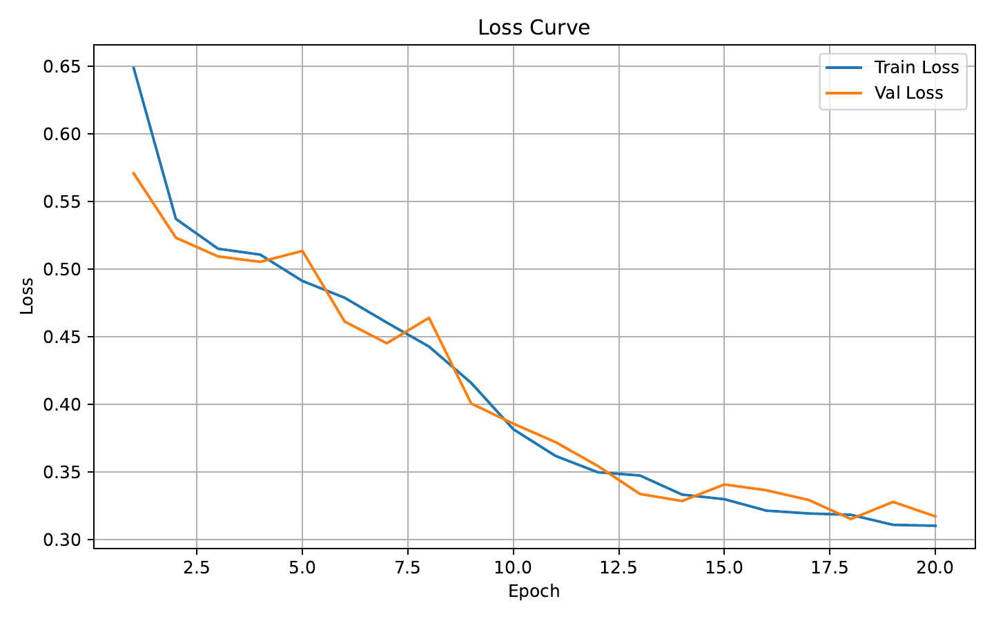
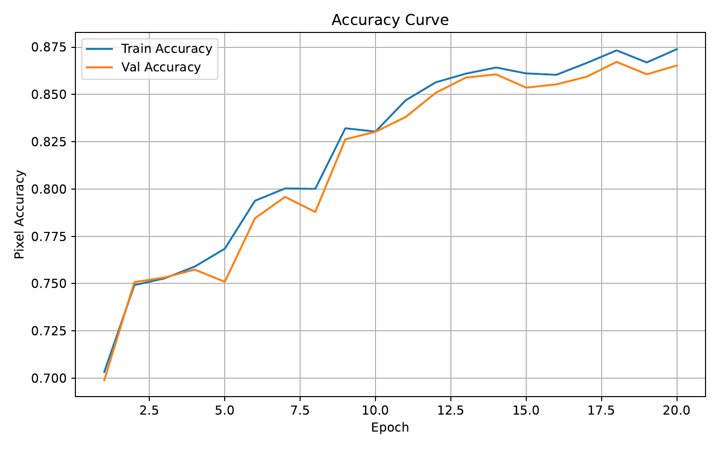
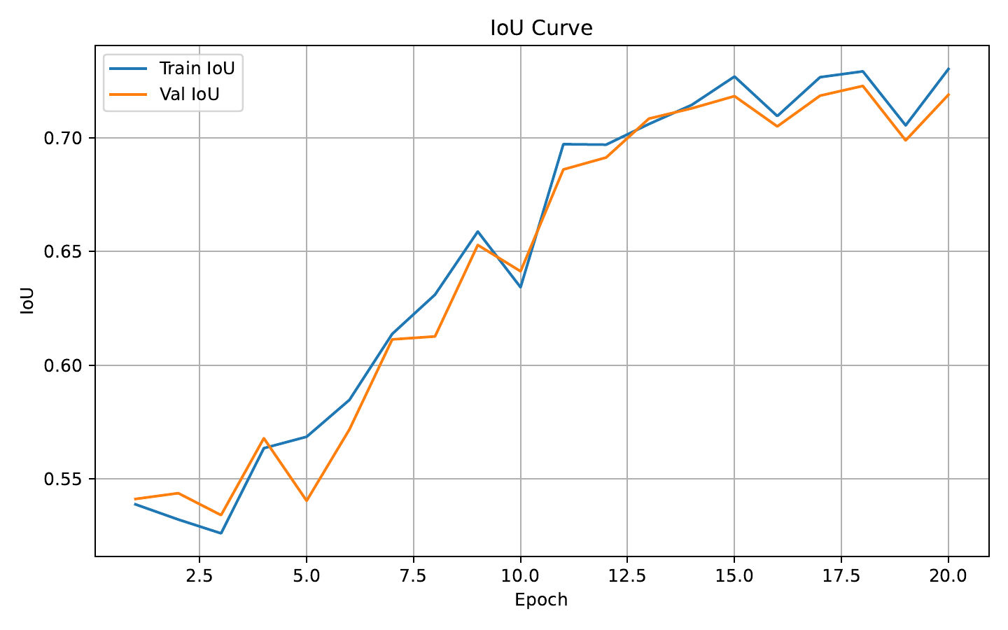
The training and validation losses decreased together over the 20 epochs, while both accuracy and IoU increased without a widening generalization gap. For this run, that behaviour is consistent with convergence without obvious overfitting.

Training dynamics

Convergence over 20 epochs

Training and validation remain close while loss falls and both segmentation metrics improve.

Measuring overlap, not only correct pixels

For predicted mask $P$ and ground truth $G$, pixel accuracy is

$$\operatorname{PA}(P,G) =\frac{\mathrm{TP}+\mathrm{TN}} {\mathrm{TP}+\mathrm{TN}+\mathrm{FP}+\mathrm{FN}} \tag{8}$$

It counts every correctly classified pixel, but can be deceptively high when background dominates the image. Intersection over Union removes true negatives from the calculation and focuses directly on foreground overlap:

$$\operatorname{IoU}(P,G) = \frac{|P \cap G|}{|P \cup G|} = \frac{\mathrm{TP}} {\mathrm{TP}+\mathrm{FP}+\mathrm{FN}} \tag{9}$$

The evaluation computes both metrics for every validation image. For scores $m_1,\ldots,m_M$, it reports not only the sample mean but also the dispersion

$$\bar m=\frac{1}{M}\sum_{i=1}^{M}m_i, \qquad s_m=\sqrt{\frac{1}{M}\sum_{i=1}^{M}(m_i-\bar m)^2} \tag{10}$$

This matters because two methods with the same average may have very different failure profiles.

def compute_iou(preds, masks, eps=1e-7):
    intersection = (preds * masks).sum()
    union = preds.sum() + masks.sum() - intersection
    return ((intersection + eps) / (union + eps)).item()

Interpreting the distributions

Per-image results

Validation-score distributions

The histograms show what the averages conceal: GrabCut has more severe failures, especially in IoU.

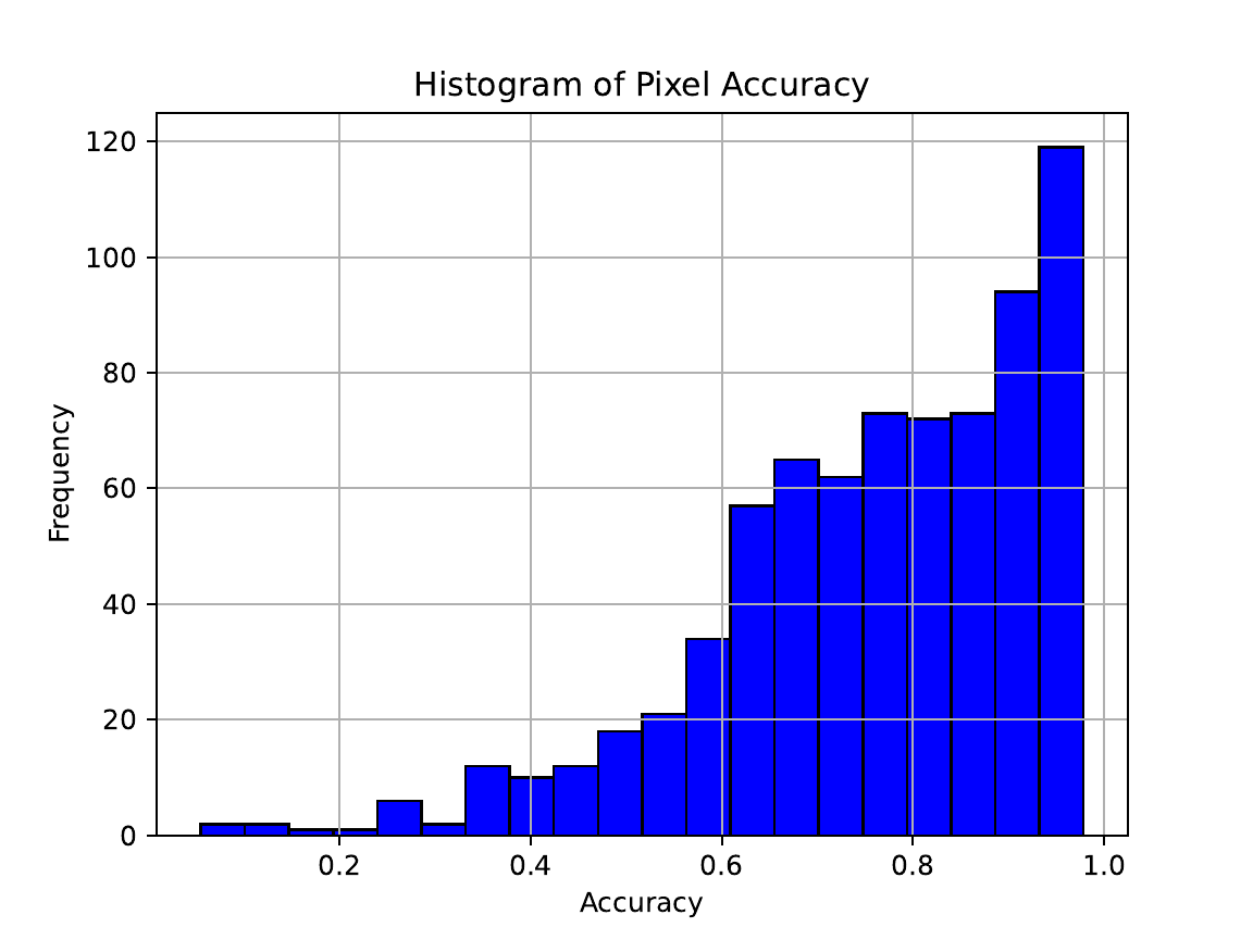
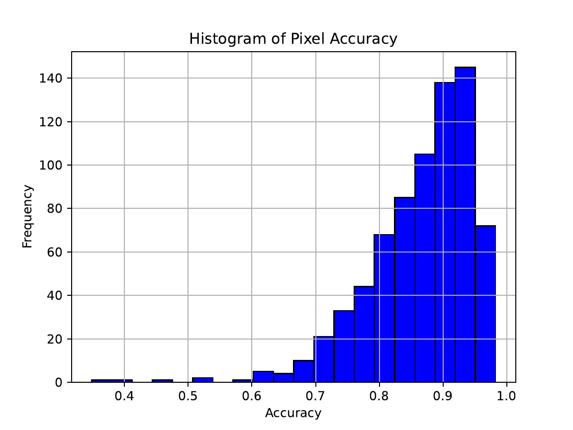
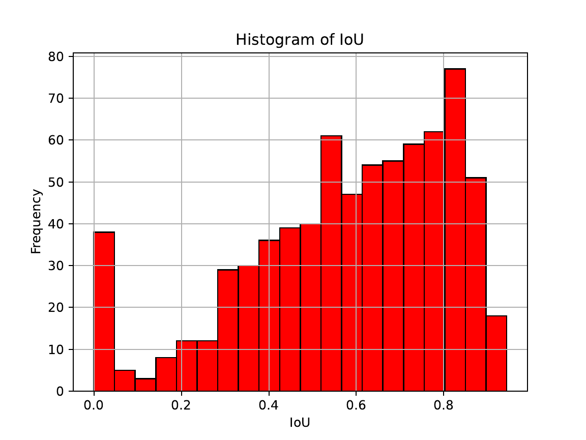
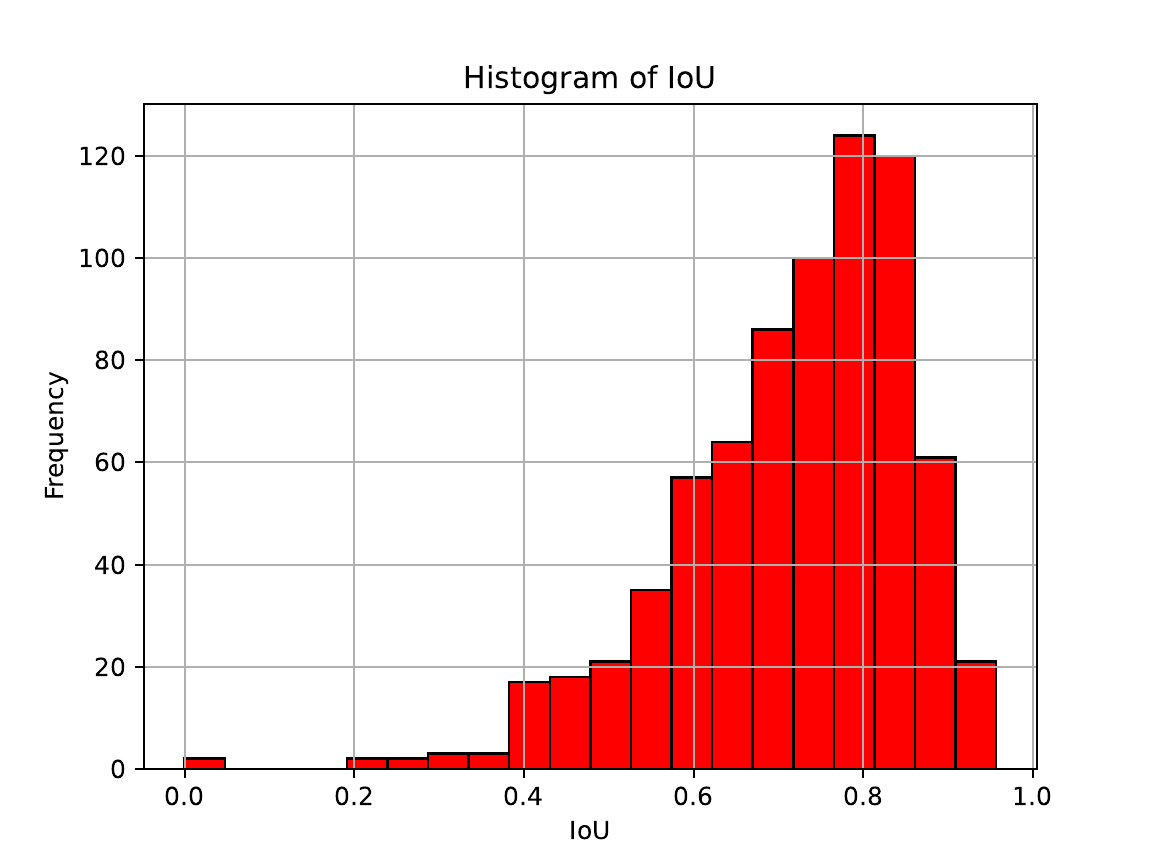
The U-Net produced more accurate and stable masks for this dataset, particularly when foreground and background colors were difficult to separate. GrabCut’s IoU distribution had a pronounced lower tail: several images received very low overlap even though the algorithm was initialized with a useful box. This is the expected weakness of a model whose principal evidence is color. When pet and background share similar distributions, the unary term becomes ambiguous and the smoothness prior cannot reconstruct semantic shape.

The network’s scores were more concentrated around their mean. Its convolutional features can represent texture, contour, and larger spatial context rather than relying on RGB similarity alone. The improvement is consequently strongest in IoU, the metric most sensitive to missing or extraneous foreground regions.

Qualitative inspection

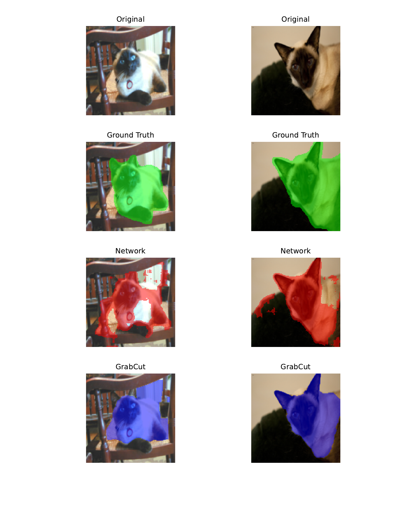
Two images, four views

Top to bottom: original image, ground truth, U-Net prediction, and GrabCut result. The network recovers the overall shape more reliably, although its boundaries remain imperfect at 128 × 128.

The actual engineering trade-off

The result is not that classical segmentation is obsolete. GrabCut is simple to deploy, needs no training set, and has no learned weights to store. For an embedded or one-off interactive system, those properties can matter more than the average metric. The U-Net is preferable when segmentation quality and consistency justify the additional training and inference cost.

Property	GrabCut	Lightweight U-Net
Prior information	Bounding box per image	Labelled training set
Optimization	Iterative, at inference time	Performed during training
Learned state	Two image-specific color GMMs	Shared convolutional weights
Main evidence	Color likelihood and local smoothness	Learned multiscale features
Deployment cost	Low storage, CPU-friendly	Model storage and tensor inference
Typical failure	Similar foreground/background colors	Distribution shift or insufficient training data

Reproducible pipeline

The repository separates data loading, both methods, evaluation, and visualization. The complete experiment can be reproduced in four explicit stages:

python methods/deep.py --mode train --plot
python methods/deep.py --mode predict
python methods/classical.py --all
python evaluation/evaluate.py

Predicted masks from both methods are written to disk before evaluation, ensuring that metric computation is decoupled from training and inference.

Limits of the study

The comparison uses binary masks at a low spatial resolution, one dataset split, and a compact network trained without data augmentation. GrabCut also receives a bounding box computed from the annotation, so its evaluation assumes an external source of object localization. These choices kept the experiment feasible on limited hardware, but they also define the scope of its conclusions.

References

1. C. Rother, V. Kolmogorov, and A. Blake, “GrabCut: Interactive Foreground Extraction Using Iterated Graph Cuts,” ACM Transactions on Graphics, vol. 23, no. 3, pp. 309–314, 2004.
2. O. Ronneberger, P. Fischer, and T. Brox, “U-Net: Convolutional Networks for Biomedical Image Segmentation,” in Medical Image Computing and Computer-Assisted Intervention, pp. 234–241, 2015.
3. O. M. Parkhi, A. Vedaldi, A. Zisserman, and C. V. Jawahar, “Cats and Dogs,” in IEEE Conference on Computer Vision and Pattern Recognition, pp. 3498–3505, 2012.
4. D. P. Kingma and J. Ba, “Adam: A Method for Stochastic Optimization,” in International Conference on Learning Representations, 2015.
5. A. Paszke et al., “PyTorch: An Imperative Style, High-Performance Deep Learning Library,” in Advances in Neural Information Processing Systems 32, 2019.