Fiducial Marker Tracking for UAVs

This project, developed at ITA with Marcos Sousa and Victor Bastos, explores a small but important part of autonomous landing: keeping track of a visual reference even when the detector briefly loses it. A camera observes a fiducial marker, YOLOv8 supplies its image-plane position, and a Kalman filter turns those intermittent measurements into a continuous estimate.

The prototype does not control an aircraft. It studies the perception layer that could precede guidance and control in an eVTOL or UAV landing system.

System structure

Each video frame passes through three stages:

Detection. YOLOv8 returns the bounding box of the marker.
Measurement. The centre of that box becomes $z_k=(c_x,c_y)^{\mathsf T}$ .
Estimation. The Kalman filter predicts the next position and corrects it whenever a new detection is available.

The distinction between detection and estimation is essential. YOLO reasons from the current image only. The filter carries a dynamical state across frames, so it can smooth noisy centres and propagate the trajectory during a short occlusion.

Tracking demonstration

YOLO detectionpredictioncorrected estimate

YOLOv8 detections feed the Kalman filter. When the marker disappears, the prediction continues to estimate its position.

Training history over 25 epochs: losses, precision, recall, and mAP.

Normalized confusion matrix for the single-class detector.

Training the detector

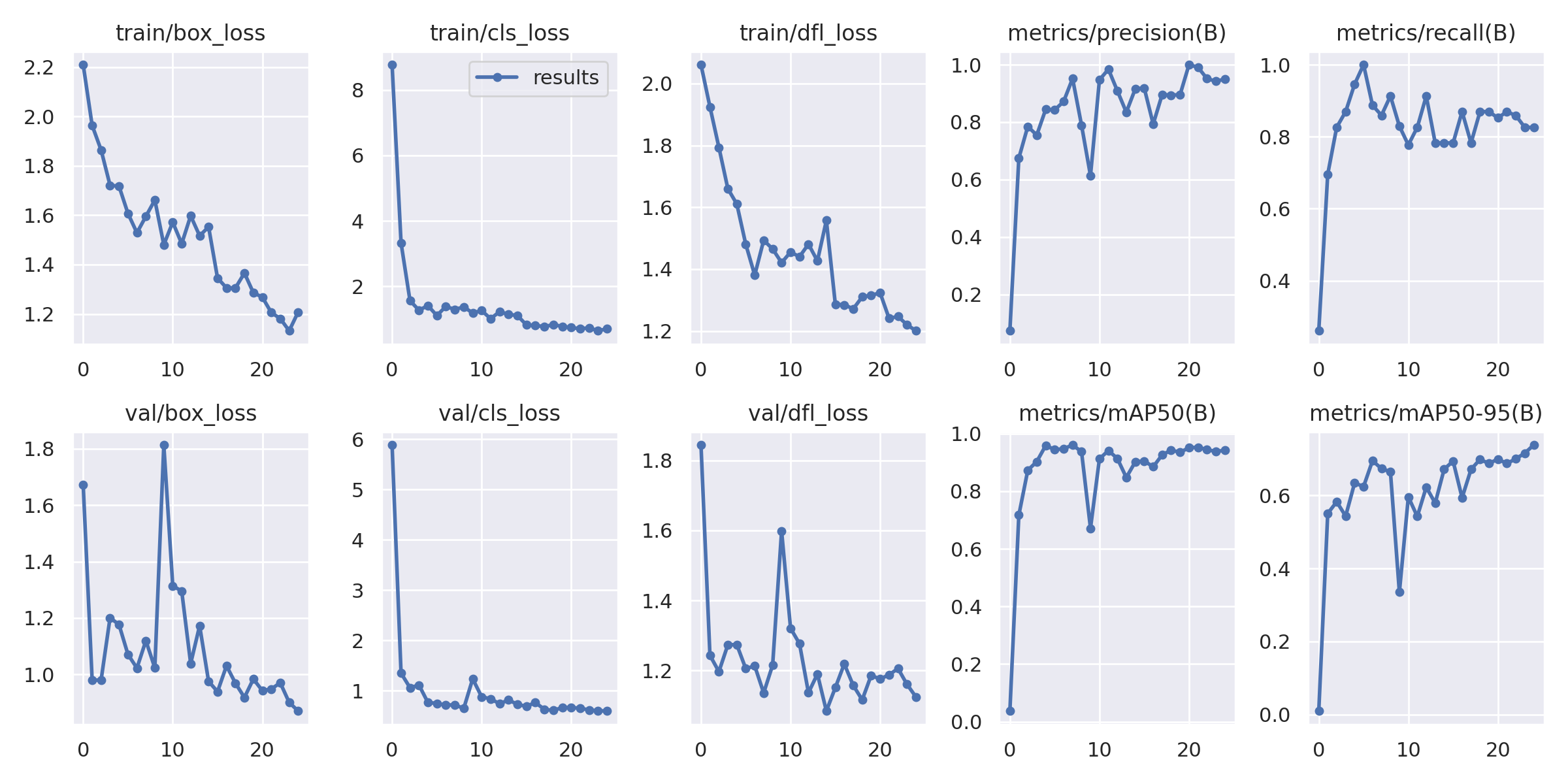
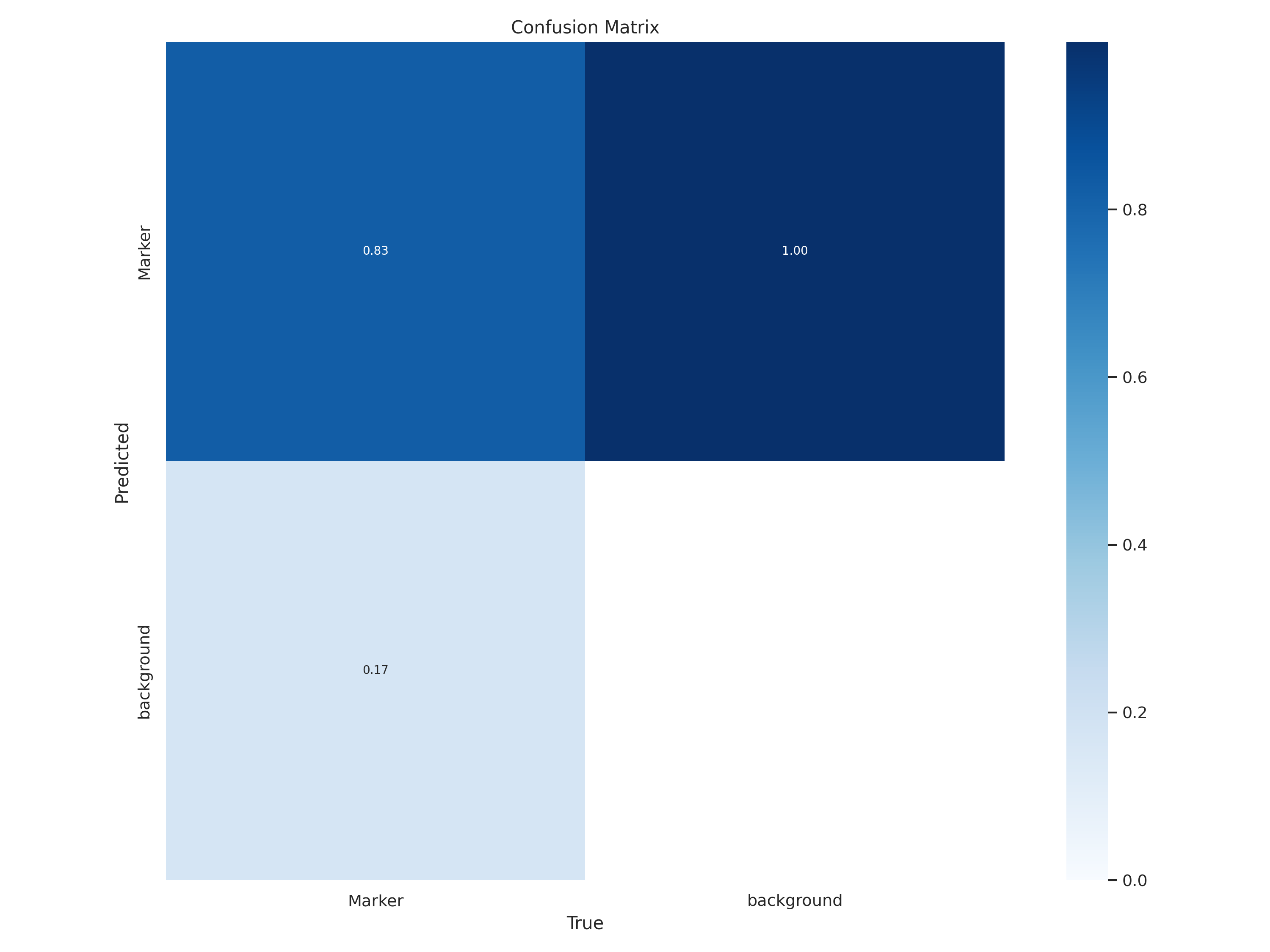
The custom dataset contains roughly 200 photographs of the landing marker captured with a phone at different distances, orientations, and lighting conditions. The notebook records 162 training images and 15 validation images, with a separate eight-image test sample. Every annotation belongs to one class: Marker.

Training used a pretrained YOLOv8s model for 25 epochs. Images requested at $185\times185$ pixels were padded by the implementation to $192\times192$ ; the batch size was 16 and optimization used SGD. Transfer learning was appropriate here because the dataset was too small to learn useful visual features from scratch.

One recorded validation run reported precision $0.950$ , recall $0.826$ , $\operatorname{mAP}_{50}=0.942$ , and $\operatorname{mAP}_{50:95}=0.733$ . These figures show that the marker was learnable, but the validation set is small enough that they should be read as prototype results rather than a deployment guarantee.

The detector reduces every retained bounding box to its centre:

results = self.model.predict(source=image, conf=0.45)

for box in results[0].boxes:
    x1, y1, x2, y2 = box.xyxy[0]
    centers.append(((x1 + x2) / 2, (y1 + y2) / 2))

That compression is deliberate: the estimator tracks a two-dimensional point, not the marker scale or orientation.

The state model

The filter uses a constant-velocity state

\mathbf{x}_k= \begin{bmatrix}p_{x,k}&p_{y,k}&v_{x,k}&v_{y,k}\end{bmatrix}^{\mathsf T} \tag{1}

with discrete dynamics and a position-only observation:

\mathbf{x}_k=A\mathbf{x}_{k-1}+B\mathbf{u}_k+\mathbf{w}_k, \qquad \mathbf{z}_k=H\mathbf{x}_k+\mathbf{v}_k \tag{2}

where

A= \begin{bmatrix} 1&0&\Delta t&0\\ 0&1&0&\Delta t\\ 0&0&1&0\\ 0&0&0&1 \end{bmatrix}, \qquad H= \begin{bmatrix}1&0&0&0\\0&1&0&0\end{bmatrix} \tag{3}

The covariance matrices $Q$ and $R$ encode two different uncertainties: how closely the marker motion follows the assumed model, and how noisy the detector centres are.

Before looking at the current frame, the filter predicts

\hat{\mathbf{x}}_k^- = A\hat{\mathbf{x}}_{k-1}^+ + B\mathbf{u}_k, \qquad P_k^- = AP_{k-1}^+A^{\mathsf T}+Q \tag{4}

When YOLO supplies a centre, the innovation $\mathbf{r}_k$ measures the disagreement between observation and prediction. The Kalman gain balances that disagreement according to their uncertainties:

\begin{aligned} \mathbf{r}_k &= \mathbf{z}_k-H\hat{\mathbf{x}}_k^-,\\ S_k &= HP_k^-H^{\mathsf T}+R,\\ K_k &= P_k^-H^{\mathsf T}S_k^{-1} \end{aligned} \tag{5}

The corrected estimate is then

\hat{\mathbf{x}}_k^+=\hat{\mathbf{x}}_k^-+K_k\mathbf{r}_k, \qquad P_k^+=(I-K_kH)P_k^- \tag{6}

If the detector returns nothing, the correction is skipped. The predicted state remains available, which is precisely the behaviour visible during the marker’s temporary disappearance in the demonstration.

prediction = kf.predict()

if centers:
    measurement = np.array(centers[0]).reshape(2, 1)
    corrected = kf.filter(measurement)

What the prototype establishes

The experiment demonstrates the intended qualitative behaviour: detections remain usable across changes in angle and illumination, the filtered point converges toward the measurements, and the motion model bridges short gaps. It also makes the system boundary clear. Detection answers where does the image suggest the marker is now? State estimation answers given that evidence and the recent trajectory, where is it most plausibly now?

The current implementation is intentionally limited. It follows the first detected centre and has no multi-object association or statistical gating. The sampling interval and acceleration input are fixed rather than derived from frame timing, and frames containing a detection advance the prediction twice in the original loop. Finally, tracking was evaluated visually rather than with trajectory error or occlusion-specific metrics.

A stronger next version would use measured timestamps, one prediction per frame, confidence-aware updates, Mahalanobis gating, and a recorded ground-truth trajectory. It could then compare raw detection error with filtered error as occlusion duration increases—and provide evidence suitable for integration with a landing controller.

References

G. Jocher, A. Chaurasia, and J. Qiu, Ultralytics YOLO, 2023.
R. E. Kalman, “A New Approach to Linear Filtering and Prediction Problems,” 1960.