Genetic PID Tuning — Leonardo Dias

This project, developed at ITA with André Thiessen and José Ronaldo, asks a concrete control-design question: what changes when the PID gains are treated as an optimization problem rather than obtained from an empirical tuning rule?

The experiment implements both approaches in Python and compares their closed-loop step responses on the same third-order plant. Ziegler–Nichols supplies a deterministic baseline from the stability boundary; the genetic algorithm searches directly for gains that score well under selected time-domain criteria.

The controlled system

The open-loop plant is

G(s)=\frac{20}{s^3+32s^2+140s} =\frac{20}{s\left(s^2+32s+140\right)} \tag{1}

and the parallel-form PID controller is

C(s)=K_p+\frac{K_i}{s}+K_ds =\frac{K_ds^2+K_ps+K_i}{s} \tag{2}

With unity negative feedback, every candidate gain triplet is evaluated through

T(s)=\frac{C(s)G(s)}{1+C(s)G(s)} \tag{3}

The implementation constructs precisely these transfer functions with python-control:

tf_sys = TransferFunction([20], [1, 32, 140, 0])
tf_pid = TransferFunction([kd, kp, ki], [1, 0])
closed_loop = (tf_sys * tf_pid).feedback()

Ziegler–Nichols as the baseline

The ultimate-gain method first removes the integral and derivative action, then increases proportional gain until the closed loop reaches sustained oscillation. For this plant, the characteristic polynomial under proportional gain $K$ is

D(j\omega)=(j\omega)^3+32(j\omega)^2+140j\omega+20K \tag{4}

Separating real and imaginary parts gives

\omega_u=\sqrt{140}\approx11.83\ \mathrm{rad\,s^{-1}}, \qquad K_u=224, \qquad T_u=\frac{2\pi}{\omega_u} \tag{5}

The classic PID rule then sets

K_p=0.6K_u, \qquad K_i=\frac{K_p}{T_u/2}, \qquad K_d=K_p\frac{T_u}{8} \tag{6}

yielding the recorded baseline $(K_p,K_i,K_d)=(134.400,505.733,8.929)$ . It is quick to compute, but the resulting loop is intentionally aggressive: its quarter-amplitude-decay character appears here as a large initial overshoot.

Encoding controller gains as chromosomes

The genetic algorithm represents $K_p$ , $K_i$ , and $K_d$ with five bits each. A chromosome therefore contains 15 bits,

\chi=\left[\chi_p\mid\chi_i\mid\chi_d\right]\in\{0,1\}^{15} \tag{7}

and each five-bit block is decoded into $[0,100]$ :

K_j=100\frac{\operatorname{int}(\chi_j)}{2^5-1}, \qquad j\in\{p,i,d\} \tag{8}

This creates only 32 possible values per gain, separated by $100/31\approx3.2258$ . The final gains— $67.742$ , $3.226$ , and $32.258$ —are exact grid points of that representation. The encoding therefore does more than store a candidate: it defines the resolution of the search.

value = np.dot(bits, [2 ** (n_bit - j - 1) for j in range(n_bit)])
value /= (2**n_bit) - 1
gain = lower_bound + (upper_bound - lower_bound) * value

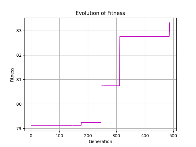
The run begins with 100 random candidates. At each generation it selects the two fittest individuals, swaps the first half of their chromosomes, mutates bits independently, evaluates the two children, and replaces the two weakest members of the population. Search stops when the best fitness exceeds 83.

What the objective rewards

Four quantities are extracted from the simulated step response: rise time $t_r$ , final value $y_\infty$ , overshoot $M_p$ , and settling time $t_s$ . The implemented score is an arithmetic mean,

J=\frac{1}{4}\left( \frac{100}{t_r+1} +\frac{100}{y_\infty+0.1} +\frac{100}{M_p+1} +\phi(t_s) \right) \tag{9}

with $\phi(t_s)=100$ for $t_s\leq10$ and $100/(t_s+0.01)$ otherwise. Higher fitness is better. This custom objective strongly rewards fast rise and low overshoot, while treating every settling time below ten seconds equally.

There is an important implementation detail: the second term uses the final output value, despite being labelled as steady-state error. For a unit step, the error should instead be $e_{ss}=|1-y_\infty|$ . The recorded controllers both reach one, so this does not distinguish their final errors in the reported comparison, but correcting the definition would make the objective mathematically consistent.

Experimental result

Metric	GA	ZN
K_p	67.742	134.400
K_i	3.226	505.733
K_d	32.258	8.929
Rise time	0.073 s	0.112 s
Overshoot	1.033%	61.805%
Settling time	0.915 s	1.900 s
Steady-state error	0	0

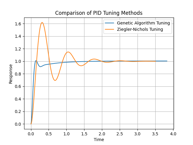
Step responses of both controllers on the same closed-loop plant.

Best fitness improves in discrete steps until it crosses the stopping target of 83.

The GA-tuned controller reached the target with approximately $1.03\%$ overshoot, compared with $61.81\%$ for Ziegler–Nichols. Its settling time was also reduced from $1.90$ s to $0.92$ s. Both responses converged to the unit reference.

These results establish that, for this plant and this objective, direct numerical search found a less oscillatory controller than the empirical baseline. They do not establish that genetic tuning is universally superior. Ziegler–Nichols was designed to provide an inexpensive initial setting, while the GA spent hundreds of generations repeatedly simulating the plant and was assessed on the same objective it optimized.

Limits and a stronger next experiment

The reported result comes from one stochastic run, one plant, and one fixed encoding. The algorithm uses a very high per-bit mutation probability, always chooses the two best parents, and does not report repeated-run variance. The objective also has discontinuities and does not penalize control effort or actuator saturation.

A stronger evaluation would repeat the search across random seeds, reserve unseen plants or perturbations for validation, and compare against modern deterministic optimizers as well as Ziegler–Nichols. An objective such as ITAE with explicit penalties for overshoot, control energy, and robustness margins would better reflect engineering requirements. Real-valued chromosomes or local refinement could then remove the quantization imposed by the five-bit encoding.

References

J. G. Ziegler and N. B. Nichols, “Optimum Settings for Automatic Controllers,” Transactions of the ASME, vol. 64, pp. 759–768, 1942.
J. H. Holland, Adaptation in Natural and Artificial Systems, University of Michigan Press, 1975.
K. J. Åström and T. Hägglund, Advanced PID Control, ISA, 2006.